 |
| Histogram of the Natural Jenks |
Tuesday, April 3, 2012
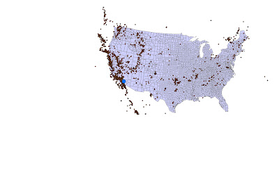
This exercise was using exploratory data with the use of Mean, Median, Standard Deviation and Variance from points taking of earthquake data.
 |
| This is the median center which identifies the location that minimizes the overall Euclidean distance to the features in the dataset. |
Wednesday, March 14, 2012
 |
| This is the study area. |
 |
| I used the same step from the IDW. This the Kriging with the default settings. |
Tuesday, March 13, 2012
Unit 4 Sediment transport Index
I started out with a DEM from the CGI. This is Oakland County of Michigan.
 |
| This the Fill |
 |
| Flow Direction |
 |
| Flow Accumulation |
 |
| I added a new shapefile to create a point on the streams to get the Watershed |
 |
| Next, I used "Extract by Mask" tool from the original DEM and the Watershed |
 |
| Generated the Slope |
 |
| I used the raster calculator to put the Sediment Transport Index formula in "Power("watershedFlowAccumulation " / 22.13,0.6) * Power(Sin("Slope_Extrac1" / 0.0896),1.3) |
Monday, February 13, 2012
Watershed Lab
This lab was about learning to do the watershed.
 |
| Flow Direction |
 |
| The Flow Accumulation |
 |
| This is the Flow Accumulation with the streams greater than 3,000 using the raster calculator. |
 |
| Flow Length |
 |
| Added my own point shapefile to go right on top of the streams. This created Pour points for areas of interests. The colored portion are the watersheds that go through the pour points. |
 |
| Behold! I also used model builder. It shows all the steps I took. |
Wednesday, January 25, 2012
Assignment 2
In this assignment, Wine
flavors are directly influenced by factors related to where the grapevines
grow, especially soil, climate, elevation, slope, and slope aspect. We wanted to find the suitable sites for a winery and
vineyard areas.
 |
| We first started with the base map. |
 |
| Then I put the elevation layer of the site of interest on to the base map. |
 |
| I used the Aspect tool, to show where the sunlight is coming from. The South and the Southwest locations that have an aspect between 157.5 and 247.5 degrees are optimal for maximum sun exposure. |
 |
| This is the slope. The green and yellow areas of the slope raster represent gentle terrain, while the orange and red areas represent steeper areas. |
 |
| In this one, I had to manually recalculate the aspect from the previous one to get them into a ranking scale of 1 to 5, with 1 being least suitable and 5 being the most suitable. |
 |
| This time I reclassified the distance to the freeways. |
 |
| And here too, I reclassified the slope. |
First Class Assignment
I used ArcGIS 10 to do these along with the Spatial Analysis tools.
 |
| First, I calculated the Slope for the surface of Wayne County, MI |
 |
| Then, I calculated the profile curvature of Wayne County |
 |
| The hillside also was calculated. |
 |
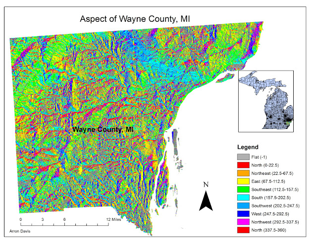
| The Aspect tool was used to show the direction of the sunlight that hit the surface in this map |
 |
| And lastly, I converted the DEM into a 3D TIN and this was the result. Since this is Wayne County, the surface is relatively flat, so not much is shown; at least in 3D. |
Subscribe to:
Comments (Atom)


